17 Feb 2016

Johnnes Kepler & his 3 laws of Planetary motion

Johannes Kepler was born in 1571 at Weil der Stadt in Wurttemberg. His mother Frau Kepler had occult leanings and must have looked exactly like a witch. In fact, at a later stage she was actually accused of witchcraft, and Johannes had a great deal of trouble in securing her acquittal.
 
However, Frau Kepler did one good deed. In 1577 she took her son outdoors to show him a bright comet (the one which Tycho Brahe saw), and from that moment on the boy was enth­ralled by astronomy.
In 1589 he arrived at the University of Tubingen to study theology. It was here that he became a convinced Copernican, and he was quite open about his views. In 1596 he wrote a book which contained some good ideas, plus a great deal of fantasy; for example he believed that each planet must have a "sphere" or band in space in which it was always to be found, and that these must touch each other, so that they could be linked with the five regular solids of geometry!
Please click on the images to enlarge


Fortunately Tycho, in Prague, read the book and liked it. He invited Kepler to join him, and Kepler did so. On Tycho's death Kepler replaced him as Imperial Mathematician, and inherited all the Hven observations, though not without opposition from some of Tycho's family.

Kepler set out to give a final solution of the problem of the planetary motions. He had total faith in Tycho's observations, but for a long time he could not make the positions of the planets fit in with any theory. Finally he realized the truth. The planets do indeed move around the Sun—but they do so not in circles, but in ellipses. From this he was led on to draw up his three Laws of Planetary Motion, which are as follows:

1. A planet moves round the Sun in an elliptical orbit. The Sun occupies one focus of the ellipse while the other focus is empty.

2. The radius vector—the imaginary line joining the centre of the planet' to the centre of the Sun—sweeps out equal areas in equal times. (This means that a planet. or for that matter a comet, moves fastest when closest to the Sun, and slowest when furthest away.)

 3. The cubes of the mean dis­tances of the planets of the Sun are proportional to the squares of their revolution periods (so that if you know the period, which is easy to find by obser­vation. you can also find the distance compared with that of the Earth. A complete model of the Solar System can be drawn up, and if one absolute value is known all the rest will follow.)

Law 3 is rather more complex. Essentially, it means that there is a definite relationship between a planet's sidereal period - that is to say, the time taken for it to go once round the Sun - and its mean distance from the Sun. This has proved to be very import­ant in measuring the length of the astronomical unit, or Earth- Sun distance.
 
What was done, in the 1960s, was to make an actual measure of the real distance of the planet Venus. Of course, the sidereal periods of both Venus and the Earth were already known very accurately, and in Kepler's relationship the only remaining unknown was the distance between the Earth and the Sun. We now know it to have a mean value of 92,957,000 miles. The measures were made by means of the latest radar techniques; radar pulses were bounced off Venus, and the time-lag between the transmission of the pulse and the reception of the "echo" pro­vided all the information for working out the distance of the planet. Radar is strictly a twentieth-century development, but the method was based on Kepler's Laws of 350 years earlier!

The first two Laws were published in 1609, and the third in 1618 in a book called Harmony the World, which was the unusual Mixture of brilliant science and outdated mysticism. Kepler also prepared a new set of planetary tables, which appeared in 1628—long after the Emperor Rudolphine had been deposed, but which Kepler called the Rudolphine Tables.

He died in 1630 while on a journey to try to collect some of the overdue wages owed to him.

15 Feb 2016

Photo Alert: A bright active Blazar [Mag 13.8] is now exciting Indian Astronomers

A blazar is a very compact quasar (quasi-stellar radio source) associated with a presumed supermassive black hole at the center of an active, giant elliptical galaxy. Blazars are among the most energetic phenomena in the universe and are an important topic in extragalactic astronomy.
 
Many of these exotic deep sky objects are faint, and very few are in range of amateur size telescope, however, Indian astronomers are now observing at active Blazar named OJ 287 of Mag 14 in the Constellation of Cancer, located to the left of M44 the Praesepe, which is increasing in brightness. An active jet is now coming into view and pointing in the direction of the Earth.
RA 08h 54m 54.48s DEC + 20 06' 14.40"
Astro photographers are urged to image the Blazar over the coming nights to monitor its activity as It could brighten to Mag 12.9.  If you do obtain images I would like to use them in a future program, please send them to rprarson46@yahoo.com.
Please click on the images to enlarge.


The astronomers report UBVRI photometric and polarimetric observations of the BL Lac object OJ 287 made on 12 February 2016. This object was recently detected in a high activity state. The polarimetry was carried out with a two beam, broadband, three channel polarimeter attached to the 1 m Carl Zeiss telescope at Vainu Bappu, India.
 
The polarimetric observation listed against the ‘R' band was made in integrated light in the VRI spectral region. The Visual mag and the broadband colours obtained are: V = 14.4, U-B = -0.50, B-V = 0.50, V-R = 0.40, V-I = 1.70. The uncertainty in Visual is around 0.1 mag, while that of a broadband colour is around 0.05 mag.


The Indian astronomers also report the temporal brightness variation of OJ 287 on the same night. The photometric observations were made in R band with a TEK 1k x 1k CCD camera attached to the 0.75-m telescope at VBO. Differential R magnitudes of OJ 287 with respect to a comparison star (J2000.0: R.A.= 08:54:54.48, Dec.=20:06:14.40; R = 14.34 mag).
 
OJ287 has been monitored in the optical wavelength with small telescopes since the beginning of September, 2015. In November and December, an unprecedented outburst in the optical band was noticed, with OJ287 reaching 12.9 mag in the Red filter. This outburst, with a possible significant thermal component, was followed by two flares of smaller amplitudes with maxima occurring on Dec 22, 2015 and January 12, 2016, originating in the jet.
The renewed optical activity of OJ287 that started on February 5. 2016. The Brightness of OJ287 rapidly rose from about 15 Mag (Feb 5) to 13.87 (Feb 10) in the R band. Most recent observation taken with PROMPT5 at 3 UT, Feb 10, indicate the target to be still increasing its brightness. On Feb 3 the degree of polarization measured using the RINGO3 polarimeter on the Liverpool Telescope was ~10%, rising to ~17% on Feb 7 and to 18-19% on Feb 8. This may also confirm the flare to be of jet origin.

13 Feb 2016

Upcoming Occultations of bright stars by the Moon

Here are the latest predictions for the occultation of bright stars by the Moon. Binoculars will show the events nicely, and a small telescope will allow you to try astronomical photography to record the events as they happen.
 
 
Below are predictions for Manila in the Philippines


11 Feb 2016

Alert bright supernovae discovered in NGC 5128


This image of nova SN2016adj was taken early this morning [11 Feb 2016].
 
RA 13h25m27.6s  DEC-43d01m09s

Supernovae explosions in distant galaxies are common, except they are usually too faint to be seen by amateur astronomers. On average they are below Mag 18 because of the immense distances involved. The most recent supernova discovery that is visible in amateur size telescopes was made on 8 February by Peter Marples using data from a 300mm F7 SCT telescope at Loganholme Observatory, Queensland, Australia. With a Mag of 14 it lies in the galaxy NGC5128 otherwise known as (Centaurus A).

The spectrum appears to be heavily reddened. The H-alpha emission line has been detected in the spectra, so the classification is consistent with a Type II supernova.
 
If you live in the southern hemisphere observations, and images, are enchouraged over the next clear evenings to track the progress of the novae before it fades from view.

I would like to include your images in my next program if I may, please send your contributions to: rpearson46@yahoo.com

Thank you for your valuable help.

Richard Pearson

10 Feb 2016

When to see Jupiter's Great Red Spot

THE GIANT PLANET Jupiter comes to opposition on 8 March, and is a splendid sight in the dawn sky.
 
At Mag -2.4 it cannot be mistaken as it lies below the main body of Leo, the celestial Lion. It's equatorial diameter is 40 arc seconds so even a small telescope will show the horizontal cloud bands, while binoculars are all that is need to show the 4 Galilean moons.
 
The most famous feature is the Great Red Spot which can be viewed in a 15 Cm (6 inch) reflector, although larger telescopes will show it clearer. It lies in the southern edge of the South Equatorial Belt.
 
Jupiter rotates quickly in about 9 hours 50 minutes so the Red Spot, which is located at 240 degrees longitude, transits over the central meridian twice every Jovian day.
 
Here are the times that the Great Red Spot can be seen on the planet's meridian from three observer stations around the Earth. All times are U.T.
 
Please bare in mind that an astronomical telescope turns the view of Jupiter upside-down so look for the red spot on the upper equatorial belt. Please click on the images to enlarge.


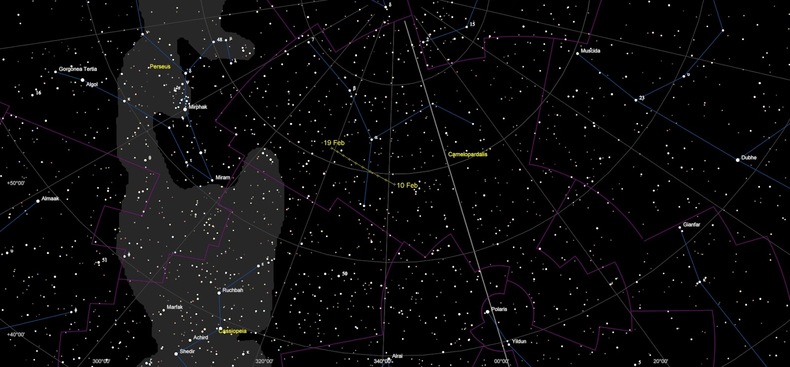
Where to find comet Catalina US10 [Mag 7]

Comet Catalina US10 is now a Mag 7 green fuzz-ball moving through the northern constellation of Camelopardalis. It continues to be at the centre of attention, an makes an ideal photo opportunity. Click on the images to enlarge.


Where to see Comet Panstarrs X1 [Mag 8]

Comet C/2013 Panstarrs X1 continues to fluctuate around Mag +8 and is now visible in the dawn sky. It lies to the south of the Great Square of Pegasus, and is moving southward into the neighbouring constellation of Pisces.  The forecast magnitude for this comet is presently 13 so it has brightened considerably.
 
Here are 2  star charts to help you locate the comet. Please click on the images to enlarge.


Variable Star alert V694 Monoceros

Star: V694 Mon
RA 07h 25m 51.28s DEC -07 44’ 08.09”
Click on images to enlarge.
 
Astronomers at the INAF-Osservatorio Astronomico di Padova in Italy are studying the unique symbiotic binary V694 Monoceros which is now on a steep rise in brightness. Indications are that it is about to surpass the record level attained during the last, and much studied, outburst of 1990, which was the brightest event in the historical light-curve of the object. At that time V694 attracted special interest by showing deep and broad absorptions, blue-shifted by 6000 km/s and completely detached from corresponding emission lines, as if originating in discrete blobs, ejected from the central star and rapidly accelerated to large velocities.
These absorptions have shown considerable variability in intensity, profile and velocity over the years. These latest measurements for February 5.967 UT shows V694 at Mag 8.88. For comparison, the peak brightness in 1990 was reached at Mag 9.2.
 
On February 5 the astronomers collected spectra on V694, in low resolution with the Asiago 1.22m telescope and in high resolution Echelle mode with the Multi Mode Spectrograph on the Varese 0.61m telescope. On top of an A-type hot continuum (with Balmer continuum in absorption), two types of absorption and two types of emission lines were observed. The absorptions in NaI D1-D2, CaII H-K, HeI 5876, and FeII multiplet 42 are located at -1900 km/s, 200-300 km/s wide, with a round profile and are completely detached from the corresponding emission lines.

The Anniversary of Stellar Specroscopy

William Huggins and his Spectroscopes


This is a memorable 'anniversary day'. On 7 February 1824 William Huggins was born. He was never a professional astronomer; he had to enter the family drapery business, and it was only when he was able to retire from the firm that he was able to devote his whole time to astronomy.
He set up an observatory at Tulse Hill, in outer London, and concentrated on astronomical spectroscopy. A spectroscope splits up light, and a normal star produces a rainbow band crossed by dark lines, each of which is the trade­mark of some particular element or group of elements. Huggins found that the stars could be divided into definite types according to their colours; a red star showed a spectrum very different from that of a white star - so that, for example, the orange Pollux has a spectrum which is easily distinguished from that of a white star such as Castor. Similar work was being carried out in Italy by the Jesuit astronomer Angelo Secchi, and the stars were put into four distinct classes (the more detailed Harvard classification system came much later):
I                       White or bluish stars, with broad, dark spectral lines due to hydrogen. Example: Sirius.
II                     Yellow stars; hydrogen lines less prominent, but more evidence of lines due to metals. Examples: Capella, the Sun.
III                    Orange stars, with complicated banded spectra. Example: Betelgeux.
IV                    Red stars, with prominent lines due to carbon. All were below magnitude 5, and many of them were found to be variable. R Cygni in the Swan was a good example.
 
What about the nebulas? Some, such as the Great Nebula in Andromeda, seemed to be made up of stars, but others, such as the nebula in Orion's Sword, looked more like patches of gas. Huggins knew that he could find out. The spectrum of a shining gas at low pressure does not yield a rainbow; instead, it produces isolated bright lines. When Huggins examined nebulae such as Orion's Sword, he saw only bright lines - and this proved that the nebulae themselves were indeed gaseous. On the other hand, the spectra of'starry nebulae' proved to be made up of the combined spectra of many millions of stars. We now know that they are galaxies in their own right, far beyond the Milky Way.
 
William Huggins died on 12 May 1910 at the age of 86.

T Tauri stars and Extrasolar Planets

The Universe According to Richard Pearson

 
We are on the eve of a truly historic occasion, because physicists are about to announce the detection of Gravitational Waves (if the recent hype can be believed). I can remember a similar occasion that occurred 30 years ago, and I also sense the rising excitement as we await the announcement on Thursday.
Back in 1981 I had a 15 Cm reflector and my main interest was variable stars. At that time extrasolar planets were in the future, and the Infrared Astronomical Satellite, IRAS, was two years away from launch.

For a number of years there was conversation among amateur and professional astronomers about T Tauri type stars because they displayed a peculiar nature, which was a bit of a mystery.
T Tauri is a variable star in the constellation Taurus. It was discovered in October 1852 by English astronomer John Russell Hind. T Tauri appears amongst the Hyades cluster, not far from Epsilon Tauri. Like all T Tauri stars, it is very young, being only a million years old. Its distance from Earth is about 460 light years, and its apparent magnitude varies unpredictably from about 9.3 to 14.

Importantly, they are generally found near molecular clouds, and T Tauri stars are pre-main-sequence, about 3 times more massive than our Sun, in the process of contracting onto the main sequence as seen in the famous HR Diagram.
Careful analysis of the star’s variable observations suggested that T Tauri itself was associated with a Protoplanetary disk, a young alien solar system in the process of formation. However, there was no evidence, and Infrared astronomy was then in its infancy.

In 1983 IRAS -- The Infrared Astronomical Satellite -- was launched into Earth orbit; it was the first observatory to perform an all-sky survey at infrared wavelengths. It imaged the star Beta Pictoris, and resolved a Protoplanetary disk for the very first time. As infrared techniques improved more discoveries of circumstellar disks followed. So T Tauri itself holds a special place in the history of extra solar planets.
Since 1988 over 2000 exoplanets have been discovered, and with better infrared telescopes, more are being added to the list with the passage of time.

Wanting to learn more about the topic of the discovery of alien planets around distant stars, I have begun reading ‘The Exoplanet Handbook’ by Michael Perryman, published in 2011 by Cambridge University Press. The book is extremely detailed, and covers the main discovery techniques used by astronomers along with analysis of their observations.
In the introduction Michael Perryman notes:

1 Astronomical Unit = the Earth/Sun distance of 93 million miles, or 150 milion Km.

“As of the cut-off date for this review, 2010 November 1, almost 500 exoplanets were known, with more than 50 multiple systems. Diversity continuing the trend established by the ear­liest discoveries, exoplanets does not adhere to the in­dividual or system properties extrapolated from the known architecture of the solar system.
Orbital properties vary widely. Around one third have very elliptical orbits, with e > 0.3, compared with the largest eccentricities in the solar system, of about 0.2 for Mercury and Pluto (and just 0.05 for Jupiter). More than half are around the mass of Jupiter (0.3 - 3Mj), and many of these orbit their host star much closer than Mercury orbits the Sun (0.39 AU): hot highly-irradiated giants piled up towards 0.03 AU that cannot have formed in situ. Others are located far out, at distances of 100 AU or more from their host star. Planets with orbits highly inclined to the star's equatorial plane occur frequently, some even with retrograde orbits.

“Exoplanets are being discovered around a wide va­riety of stellar types. Host stars are not only main se­quence stars like the Sun, but they include very low- mass stars, low metallicity stars, giant stars, and other advanced evolutionary stages such as white dwarfs and pulsars. Their internal structure and composition vary widely too. Gas giants with stripped outer envelopes, water worlds formed beyond the snow line, and carbon- dominated terrestrial planets may all exist. The first Exoplanet atmospheres have been probed through sec­ondary eclipse photometry and spectroscopy.
“Of the multiple Exoplanet systems, massive plan­ets orbiting in mean motion resonance are common, presenting a certain challenge to explain their ubiquity. The first triple-planet Laplace resonance has been dis­covered, as have prominent transit time variations in a two-planet transiting system. Systems with multiple lower-mass planets are being found in increasing num­bers as the radial velocity surveys improve their detec­tion threshold and increase their temporal baseline. The fire-planet system 55 Cnc has been overtaken by the (possible) six-planet system GJ 581 with a 3.1M® planet in the habitable zone, and up to seven planets with five Neptune-mass in the case of HD 10180.”
In my opinion, as we move into 2016 It will not be long before astronomers discover an Earth like planet similar to our own, and then speculation will focus on finding the tell tale signs of intelligent life. The gigantic reflector telescopes now under construction in Chile will help astronomers discover the very first Earth-like planet, and you will then be the first to witness another truly historic occasion.
Richard Pearson

9 Feb 2016

Lunar Photo opportunities to come


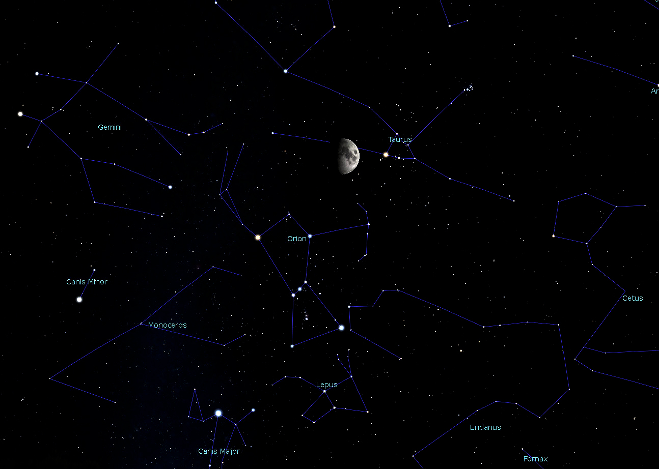
AS SOON as darkness decends on 16 February look due south and you will seen the Moon close to the Hyades open cluster, and Aldebran, the 'eye of the bull.' This is a nice photo-opportunity for astrophotographers to record.


From about 10pm (UT) on 24 February look into the eastern sky to see the Moon 2 degrees south of the lovely ringed planet Saturn, which will be nice to see with binoculars. Again this will be a good photo opportunity.

Clear skies everyone.

How do EMDrives work?

The Universe according to Richard Pearson


IT IS A VAST Cosmos out there, the nearest star to Earth, Proxima Centauri, is so far away its light takes 4.3 years to reach us travelling at the speed of light, 300,000 Km/s, while our Milky Way galaxy is 100,000 Ly across. Travelling over oceans of space requires speed and novel propulsion systems to allow spacecraft to reach speeds close to light velocity.

A radio frequency (RF) resonant cavity thruster is a proposed new type of electromagnetic thruster. Unlike conventional electromagnetic thrusters, they are designed to use no reaction mass, and to emit no directional radiation. Their design principles are not supported by prevailing scientific theories, and they apparently violate the law of conservation of momentum.

A few variations on such thrusters have been proposed. Aerospace engineer Roger Shawyer designed the EMDrive in 2001, and has persistently promoted the idea since then through his company, Satellite Propulsion Research.

Researchers say the new EMDrive could carry passengers and their equipment to the moon in as little as four hours. 


A trip to Alpha Centauri, which would take tens of thousands of years to reach right now, could be reached in just 100 years.

Last summer the controversial design for the EMDrive received a boost as German scientists confirmed that it does in fact work.

The EMDrive propulsion system would permit travel at speeds until now only seen in science fiction.

The system is based on electromagnetic drive, or EMDrive, which converts electrical energy into thrust without the need for rocket fuel. 

The concept of an EMDrive engine is relatively simple. It provides thrust to a spacecraft by bouncing microwaves around in a closed container.

Solar energy provides the electricity to power the microwaves, which means that no propellant is needed.

According to classical physics, the EMDrive should be impossible because it seems to violate the law of conservation of momentum.

The law states that the momentum of a system is constant if there are no external forces acting on the system – which is why propellant is required in traditional rockets.

But subsequent tests - further backed up by this announcement - have shown that the idea could revolutionize space travel.

Bouncing microwaves around in a ‘closed container’ is strange idea, except in it is not actually a closed container, on the Quantum scale it is open throughout, and Quantum fluctuations are happening in the container.

In quantum physics, a quantum fluctuation (or quantum vacuum fluctuation or vacuum fluctuation) is the temporary change in the amount of energy in a point in space, as explained in Werner Heisenberg's uncertainty principle. It means that conservation of energy can appear to be violated, but only for small times. This allows the creation of particle-antiparticle pairs of virtual particles. The effects of these particles are measurable, for example, in the effective charge of the electron, different from its "naked" charge.

The copper and steel of the EMDrive has a molecular structure made up of atoms, at lesser scales the atoms are composed of smaller atomic particles, and there is a lot of empty space between the orbital electrons and the nucleus.

For example, the simplest atom is that of Hydrogen, it contains one neutron, and proton that make up the central nucleus, while there is a single electron in orbit around it. If the nucleus happened to be the size of an apple, then the distance of electron would be a third of a mile distant. That is a lot of empty space on the quantum scale of our Universe.

In my opinion on this atomic scale, while the drive is closed to the vacuum of space, microwaves are not, and can interact with quantum particles surrounding the EMDrive.

The space inside the EMDrive is not empty; it contains quantum pairs of atomic particles that the microwaves can interact with.

If physicists can better understand this process, much better propulsion systems can be designed to reach light speed in a shorter time so that we can reach for the stars.

Richard Pearson


6 Feb 2016

Celebrates Astronaut Edgar Dean Mitchell


Apollo 14 was originally targeted for Taurus-Littrow but was diverted by the Apollo 13 abort to Fra Mauro. The mission was delayed for forty minutes by weather resembling the conditions for Apollo 12, and it surprised some observers to see the liftoff going ahead in very murky skies at 16:03 hrs local time. The parking orbit was 186 km (116 miles) and 32.4° inclination. The all-rookie crew in terms of orbital space flight, with only commander Alan Shepard having any space flight experience (a mere sub-orbital lob in 1961), were placed on their trans-lunar coast with no difficulty. CMP Stuart Roosa closed in for the transposition and docking but couldn't dock. A drama unfolded as Roosa tried six times, at last succeeding after 106 minutes. If the docking mechanism was faulty, the Moon landing would have to be cancelled. Once the Lunar Module Antares and Command Module Kitty Hawk were joined up, Shepard and his crew inspected the docking probe, but could not explain the earlier difficulty. NASA deliberated for a while before announcing that the Moon landing attempt would proceed.

Apollo 14 entered lunar orbit quietly, lowering its perilune to the lowest ever for the complete Apollo combination at just 16 km (10 miles). Manned by the steely-eyed Shepard and burly Edgar Mitchell, Antares separated and just before the PDI burn hit trouble. First, a short circuit in the LM computer abort switch meant the computer could not be persuaded not to abort the landing attempt. The crew just finished reprogramming themselves out of this problem when the landing radar failed. With an abort just seconds away, at which point the PDI could not bring them into the landing site, Mitchell's desperate switch flicking succeeded. Shepard brought Antares on to Fra Mauro with 40 seconds of fuel left, some 26.5 m (87 ft) off target, and at a tilt angle of 6°, at 30°40'27" south 17°27'58" west.
 
On 5 February, Shepard set foot on the Moon at T + 114 hours 31 minutes and was joined by Mitchell. The television camera was pointed at the sloping LM, with the sun very low in the sky, and it was not possible to follow the crew all the time as they set to work laying out the ALSEP instruments and collecting samples using the Modular Equipment Transporter. This was a lunar "wheelbarrow", which some of the less interested press reports suggested was to carry the aging Shepard when he got tired. The EVA lasted 4 hours 49 minutes and the second, on 6 February, lasted 4 hours 35 minutes and featured a thwarted and tetchy attempt to climb the 45 m (147.5 ft) high rim of Cone Crater. Although Shepard was convinced that they were nowhere near the rim and decided to abort the attempt, Mitchell had in fact been right in his assertion that they had nearly reached it. Shepard won the argument.
 
During the EVAs the crew had travelled about 2.72 km (2 miles) on foot, and at the end of the second EVA Shepard played his famous televised game of lunar golf, using a proper ball and a club made from the head of a 6-iron with an attachment to fit the handle of the contingency sample collector A passionate golfer, Shepard drew the ball out of his suit leg pocket and dropped it on the surface. Being limited in his mobility he sliced more lunar soil than ball in his first one handed "swing" barely moving the ball (something he was ribbed about back at the Astronaut Office after the mission). For the second attempt, a new ball was taken from the suit pocket and this time he hit it into a crater about 15 metres away. Not to be out done in this demonstration of lunar sports, Mitchell threw the staff from the solar wind composition experiment into the same crater. After 33 hours 39 minutes on the Moon, Antares lifted off and docked with Kitty Hawk, which itself leapt out of lunar orbit after a stay of 66 hours 39 minutes. The Command Module came home 6.4 km (4 miles) from the recovery ship USS New Orleans in the Pacific Ocean at 27° south 172° west at T + 9 days 0 hours 1 minutes 57 seconds - the most accurate splashdown, 600 m (1950 ft) from the predicted target. The crew was the last to have to endure the quarantine container.

5 Feb 2016

NASA Shows Off Orion Command Module for 1st Lunar Flight Test

NASA’s Orion crew module pressure vessel is secured on a test stand called “the birdcage” inside the Neil Armstrong Operations and Checkout (O&C) Building high bay at NASA’s Kennedy Space Center (KSC) in Florida. The pressure vessel makes up the underlying structure of the Orion crew module, which will be used for the agency’s unmanned Exploration Mission (EM)-1 flight in 2018. On this mission, the spacecraft will travel significantly farther and spend a much longer duration in space than the previous Exploration Flight Test (EFT)- 1 mission that took place in December 2014.
 
“This vehicle will go further than any of the Apollo spacecraft has ever went,” said Mark Geyer, John Space Center (JSC) deputy director and former Orion program manager. “It’s the beginning of this architecture, SLS and Orion, to enable us to explore the lunar regions and encounter things like a habitation module, visit asteroids, and then eventually go on to Mars. All a part of leading exploration and the United States being a leader in that.”
 
NASA’s Super Guppy aircraft transported Orion’s completed structure from the agency’s Michoud Assembly Facility in New Orleans (where it was welded together) to KSC’s Landing Facility on Feb. 1. The structure is the foundation on which all of the spacecraft’s systems and subsystems are going to be built and integrated to provide a sealed environment for astronauts to survive.
 
In order to prepare this particular spacecraft for the rigorous EM-1 mission, Orion will first undergo a series of tests to ensure it is structurally sound before spending the next 18 months getting outfitted with its necessary flight systems and subsystems, including its heat-shielding thermal protection system, before being shipped to NASA’s Plum Brook Station in Ohio to undergo a series of thermal vacuum tests prior to EM-1. More than 100,000 components will be integrated with the spacecraft by the Orion team at KSC.
 
More than 500 GB of data was gained from the EFT-1 flight to aid engineers with Lockheed Martin in constructing the first SLS Orion to fly, and one major change is the build of the primary structure itself now at KSC. Engineers reduced the number of welds for the crew module by more than half, and fewer welds means an overall lighter spacecraft (700 pounds).
 
According to NASA, the first crew module structure that was built and used for engineering tests and evaluations required 33 weld operations. The number of welds required for the Orion structure that flew EFT-1 was reduced to 19, and further innovations have reduced the welds to 15 for the EM-1 spacecraft.
 
Seven large aluminum pieces were cleaned, coated with a protective chemical, and primed to protect from corrosion before each element was outfitted with strain gauges and wiring to monitor the metal during the fabrication process. Each piece was then inspected and evaluated to ensure meeting precise design requirements before being welded together using a state-of-the-art process called friction-stir welding, which produces very strong bonds by transforming metals from a solid into a plastic-like state, and then using a rotating pin tool to soften, stir and forge a bond between two metal components to form a uniform welded joint.
 
The EM-1 spacecraft may be destined to fly the furthest mission of a human-rated vehicle in history, but it isn’t the first Orion to be built. In 2010, the first Orion flew on Pad Abort (PA)-1 to demonstrate the Launch Abort System (LAS). In 2014, the second Orion flew on NASA’S EFT-1 mission and took Orion 3,600 miles above Earth’s surface (roughly 15 times higher than the International Space Station) for a 4.5-hour orbital flight test. On EM-1, Orion will launch aboard the inaugural flight of the agency’s Space Launch System (SLS) rocket and travel nearly 40,000 thousand miles beyond the orbit of the Moon on a three-week mission to prove out the entire flight system before strapping astronauts onboard in the first half of the next decade.
 
Orion must be able to withstand high velocities and re-entry temperatures when coming back from beyond low-Earth orbit, bringing with it temperatures and velocities not seen by a crewed vehicle since moonshot days of Apollo. Orion will experience speeds as fast as 24,545 mph (39,501 km/h), or 36,000 feet per second, as the spacecraft makes its return from lunar velocity during EM-1. To put that in perspective, during EFT-1, Orion experienced a fiery re-entry at 20,000 mph (32,000 km/h), or 30,000 feet per second. At that speed temperatures soared as high as 2,200 degrees Celsius (4,000 degrees Fahrenheit) around the spacecraft, and for this reason Orion’s new thermal protection system was forced to evolve from the EFT-1 flight article.
 
While EFT-1’s heat shield surpassed expectations, changes were necessary for the actual deep-space missions. NASA and Lockheed Martin added a 3-D woven thermal protection fabric soon after EFT-1, designed to fit between Orion and the service module. Six “quartz” compression pads will serve to absorb shock during launch and spaceflight operations; during reentry, the material will serve as an ablative thermal protection system.
 
A more effective way of building the heat shield was also proposed. Orion’s outer heat shield surface will consist of 180 blocks, versus having it fabricated in one single, massive piece. The spacecraft’s back shell will be covered with a silvery, metallic thermal control coating, which will not only reduce heat loss in deep space, but will also limit high temperature exposure to the crew.
 
“The heat shield we put to the test during Orion’s flight test last December met every expectation we had and gave us a tremendous amount of data on its thermal and mechanical performance,” said Mark Kirasich, Acting Orion Program Manager. “But the process of building the heat shield as a single piece for that flight also gave us insight into how we could improve the way we build this essential element of the spacecraft.”
By Talia Landman

The Moon during February

THE EMPHERMERIS INFORMATION FOR OBSERVERS OF THE MOON DURING
FEBRUARY. Top information is for Washington (US). Bottom information for Nottingham (UK).
Please click on the graphics for a larger view.
 

4 Feb 2016

The Moons of Saturn during February


Click on the images to enlarge

Saturn is the showpiece of the sky. Apart from Jupiter, it is by far the largest member of the Sun's family; even though it is so far from the Sun (886,000,000 miles on average) it shines brightly, and even a modest telescope will show its superb system of rings. Also on view will be some of the remarkably interesting retinue of moons or satellites.
I have been asked many time what size telescope is needed to see the Moons now that Saturn is at a reasonable height in the dawn sky. Here are the average magnitudes of Saturn's principal satellites.
There are 62 satellites altogether. One of them, Titan Mag 9.7, is of planetary size, and is visible with a 2-inch telescope. Of the rest, Iapetus Mag 13, Rhea Mag 9.7, Dione Mag 10.6, and Tethys Mag 10.7 are moderately bright, but the others cannot be seen except with the help of powerful instruments.
Mimas Mag 12 and Enceladus Mag 11.6 are distinctly elusive (I find them difficult even with a 12-inch reflector), but are interesting because they seem to be only about as dense as water.
Next, reckoning outward from Saturn, we come to Dione Mag 10.6, which is much more massive than Tethys. My own observations indicate that it is a little brighter, but in any case a modest telescope will show both. Rhea Mag 9.7 is further out, and larger, so that it is quite easy to see in a small instrument.
Between the orbits of Titan and the next major satellite, Iapetus, there is a wide gap. In this region Bond, in 1848, found a small moon, Hyperion Mag 13, which is distinctly difficult to observe.
All the inner moons move practically in the plane of Saturn's equator, which is the plane of the ring-system. Iapetus, however, has an orbital tilt of more than 14 degrees. It is a long way from Saturn, and its movement’s are relatively slow. But its main point of interest lies in the fact that it is variable in brightness. When west of Saturn, it is conspicuous; my observations indicate that it can become brighter than the 9th magnitude.